How does linkage disequilibrium evolve?

Because all our SNPs were independent of each other, and all the samples were unrelated, we wouldn't expect to see any strong linkage disequilibrium (correlation between genotypes at different variants) at the start of our simulation. Or do we? Let's compute the LD now and see.

Note that cor() in R computes correlations between columns, whereas np.corrcoef() in Python computes correlations between rows by default, so we use .T to transpose the haplotype matrix, equivalent to t() in R.

compute.ld <- function( haplotypes ) {
  cor( haplotypes )
}

compute.ld( haplotypes[population[1,],] )

def compute_ld(haplotypes):
    return np.corrcoef(haplotypes.T)


compute_ld(haplotypes[population[0]])

You should get a big 20x20 matrix of correlation values, with ones on the diagonal and lower values between SNPs.

Warning

You'll probably also see quite a few missing values in there. These are correlations between genetic variants - some of the genetic variants may actually be zero frequency, so there's no correlation to compute!

The image() function in R or the imshow() function in Python's matplotlib can be used to visualise this.

plot.ld <- function( haplotypes ) {
  # By default `image()` chooses its own colour set, but we'll
  # specify a fixed set using the breaks` and `col` arguments
  breaks = c( -0.01, seq( from = 0.1, to = 1, by = 0.1 ))
  ld.colours = c( 'grey95', rev( heat.colors( length(breaks)-2 )))
  r = compute.ld( haplotypes )
  image(
    r^2,
    col = ld.colours,
    breaks = breaks
  )
}

plot.ld( haplotypes[population[1,],] )

def plot_ld(haplotypes, ax=None):
  if ax is None:
      fig, ax = plt.subplots()
  # An Python equivalent to heat.colors is the autumn_r colormap
  ld_colours = plt.colormaps["autumn_r"].with_extremes(under="lightgrey")
  r = compute_ld(haplotypes)
  ax.imshow(
    r**2,
    cmap=ld_colours,
    vmin=0.1, vmax=1, origin="lower",
  )
  return ax

plot_ld(haplotypes[population[0]])

Here we've plotted r²; the colour scale is set up so red points are variants in high LD (also seen on the diagonal); yellow & orange points have intermediate LD; and grey points have r² < 0.1. And white points have missing values (which occurs if one or other of the variants was actually monomorphic.) It should look something like this:

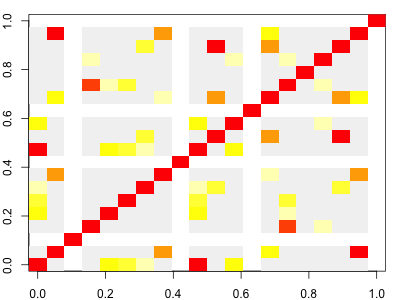
Note. As it turns out, even at this starting point in our simulation, there can be a bit of LD. It arises due to our finite set of starting haplotypes.

Now plot the LD for the final generation and compare to the original:

layout( matrix( 1:2, ncol = 1 ))
plot.ld( haplotypes[population[1,],] )
plot.ld( haplotypes[population[G,],] )

fig, axes = plt.subplots(2, 1, figsize=(6, 12))
ax = plot_ld(haplotypes[population[0]], axes[0])
ax = plot_ld(haplotypes[population[G-1]], axes[1])

Question. What do you see?

Note

Depending on your simulation, you might see interesting patterns emerging. On the other hand, you might just see lots of white (missing) LD - it depends what happened in the simulation.

Not to worry! You can always go and run the simulation again if you don't like what you see:

```r # Only run this line if you want to re-initalise the starting population: # population[1,] = sample( 1:H, size = N, replace = TRUE )

for( generation in 2:G ) { population[generation,] = evolve( population[generation-1,] ) } layout( matrix( 1:2, ncol = 1 )) plot.ld( haplotypes[population[1,],] ) plot.ld( haplotypes[population[G,],] )

```python
# Only run this line if you want to re-initalise the starting population:
# population[0] = np.random.choice(H, size=N, replace=True)


for generation in range(1, G):
    population[generation] = evolve(population[generation-1])

fig, axes = plt.subplots(2, 1, figsize=(6, 12))
ax = plot_ld(haplotypes[population[0]], axes[0])
ax = plot_ld(haplotypes[population[G-1]], axes[1])

Question. What is the simulation doing to linkage disequilibrium?