Exploring the simulations

In this file: on github (right click and choose 'Save as' to save it).

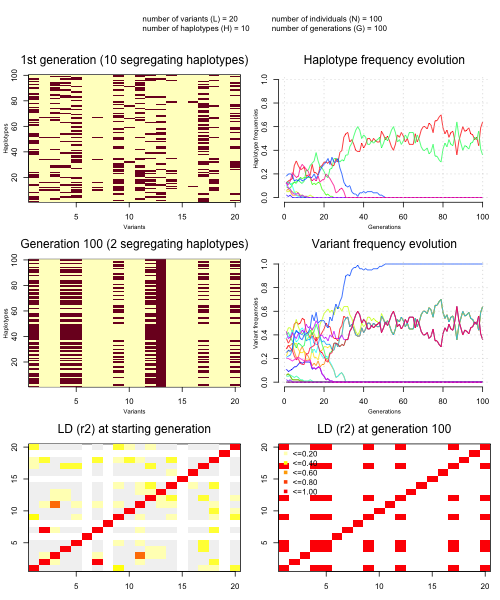
I've wrapped up the above simulation into two key functions:

• simulatePopulation() which simulates from the model as above.
• plotSimulation() which makes a multi-panel plot of the result.

To get this code, you can source() it into your session in R, or import it in Python:

source( "simulation_and_visualisation.R" )

from simulation_and_visualisation import (
  simulatePopulation, plotSimulation
)

You can run it like this:

sim = simulatePopulation( L = 20, N = 100, G = 100 )
plotSimulation(sim)

sim = simulatePopulation(L=20, N=100, G=100)
plotSimulation(sim)

or on one line:

plotSimulation( simulatePopulation( L = 20, N = 100, G = 100 ) )

plotSimulation(simulatePopulation(L=20, N=100, G=100))

It produces a plot like this:

Questions

• Explore the simulations and try varying the parameters.

How does varying the population size $N$ affect the simulations? e.g. what if you set $N = 1,000$? $10,000$?

(NB. One effect is, it's slower!)

What if you turn up $N$ to $1,000$, but also run 1,000 generations?

Describe in general what happens to haplotypes and variants as the simulations proceed.

What does genetic drift do to frequencies, and LD?

Reminder

Remember that in this simulation

• $L$ is the number of variants across the region
• $N$ is the population size,
• and $G$ is the number of generations.

In this code, if you want, you can also specify:

• $H$, the number of different haplotypes we created at the simulation start, and
• initial.frequency, the starting frequency of each genetic variant.

Next steps

Next let's look at some key population genetic statistics.