How do frequencies evolve?

If you look at the 'before' and 'after' haplotypes, you'll probably see some features:

• many variants are no longer polymorphic - the other alleles have been 'lost' or have 'fixed'
• many of the remaining alleles are either rare or common.

But how do these evolve over time? To see that let's write some quick functions to compute the haplotype and variant frequencies across time:

compute.haplotype.frequencies <- function( population, haplotypes ) {
  # We compute the frequency of each haplotype at each generation
  result = matrix(
    nrow = G, ncol = H,
    dimnames = list(
      sprintf( "generation=%d", 1:G ),
      sprintf( "haplotype=%d", 1:H )
    )
  )
  for( i in 1:G ) {
    currentGeneration = population[i,]
    result[i,] = sapply(
        1:H,
        function(h) { length( which( currentGeneration == h )) }
    ) / N
  }
  return( result )
}

def compute_haplotype_frequencies(population, haplotypes):
  # We compute the frequency of each haplotype at each generation
  G, N = population.shape
  H = haplotypes.shape[0]
  result = np.empty((G, H))

  # NB: instead of R's sapply, below we can use
  # np.bincount which efficiently counts the number
  # of 0s, 1s, 2s, 3s etc in an array
  for i in range(G):
    current_generation = population[i]
    result[i] = np.bincount(  
        current_generation,
        minlength=H,
    ) / N
  return result

And to plot them:

# Utility function to plot an empty canvas
blank.plot <- function( xlim = c( 0, 1 ), ylim = c( 0, 1 ), xlab = "", ylab = "" ) {
  plot(
    0, 0,
    xlab = xlab,
    xlim = xlim, ylab = ylab, ylim = ylim,
    col = 'white', # draw points white
    bty = 'n',     # no border
    xaxt = 'n',    # no x axis
    yaxt = 'n'    # no y axis
  )
}


plot.haplotype.frequencies <- function( frequencies ) {
  G = nrow( frequencies ) # number of generations
  H = ncol( frequencies ) # number of haplotypes
  blank.plot(
      xlim = c( 1, G*1.1 ), ylim = c( 0, 1 ),
    xlab = "Generations", ylab = "Haplotype frequencies"
  )
  palette = rainbow( H )
  for( i in 1:H ) {
    points( 1:G, frequencies[,i], col = palette[i], type = 'l' )
    if( frequencies[G,i] > 0 ) {
        text(
            G*1.02, frequencies[G,i],
            sprintf( "Hap %d", i ),
            col = palette[i],
            adj = c( 0, 1 ), xpd = NA
        )
    }
  }
  grid()
  axis(1)
  axis(2)
}

# To match the R function: take in an axes obj and format it
def blank_plot(ax, **kwargs):
  if ax is None:
    fig, ax = plt.subplots()
  ax.set(**kwargs)
  ax.spines["top"].set_visible(False)  # no axis line on top
  ax.spines["right"].set_visible(False) # no axis line on right
  return ax






def plot_haplotype_frequencies(frequencies, ax=None):
  G, H = frequencies.shape
  ax = blank_plot(
      ax, xlim=(1, G*1.1), ylim=(0, 1),
      xlabel="Generations", ylabel="Haplotype frequencies",
  )
  palette = plt.cm.rainbow(np.linspace(0, 1, H))
  for i in range(H):
    ax.plot(range(G), frequencies[:, i], color=palette[i])
    if frequencies[G-1, i] > 0:
      ax.text(
        G*1.02, frequencies[G-1, i],
        f"Hap {i+1}",
        color=palette[i],
        ha="left", va="top"
      )


  ax.grid()
  return ax

And run it:

frequencies = compute.haplotype.frequencies( population, haplotypes )
plot.haplotype.frequencies( frequencies )

frequencies = compute_haplotype_frequencies(population, haplotypes)
ax = plot_haplotype_frequencies(frequencies)

You might see something a bit like this:

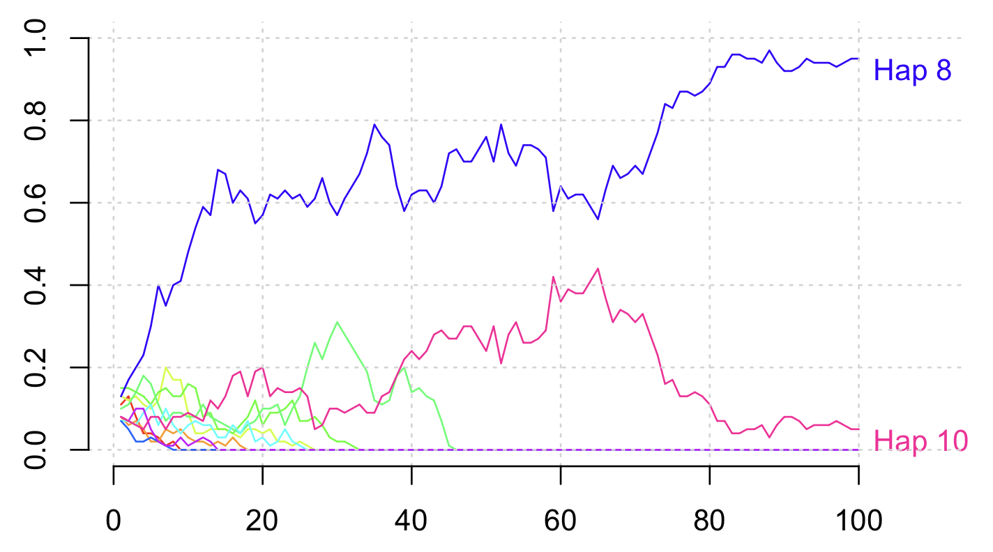
Here haplotypes 8 and 10 are present in the population at the end - the others have been lost!

But of course yours will look different - it's a stochastic simulation.

Question. What is happening to the haplotype frequencies over time? What is causing this?

Terminology

The effects of random inheritance on the evolution of haplotypes are also known as genetic drift.

You might also want to see how the alleles are spread through the population - here's another plot that shows that:

long_form = (
  expand.grid( individual = 1:N, generation = 1:G )
  %>% dplyr::group_by( individual, generation )
    %>% dplyr::mutate( haplotype = population[generation, individual] )
)

par( mfrow = c( 2, 1 ))

plot.haplotype.frequencies( frequencies )

palette = rainbow( H )
plot(
    long_form$generation,
    long_form$individual,
  xlim = c ( 1, G*1.1 ),                 # to match haplotype
    bg  = palette[ long_form$haplotype ],  # fill colour
    pch = 22,                              # filled squares
  cex = 0.5,                             # small size
    col = NA,                              # no outline on shapes
    xlab = "Generations",
    ylab = "Individual",
    bty = 'n'                              # no border
)

Hmm!