Sanity check!

Another good idea is to check whether our model really fits the data.

Here's a good way to do that - plot theoretical versus observed frequencies.

observed_frequencies = (
    full_data
    %>% group_by( sum_of_dice )
    %>% summarise(
        n = n(),
        frequency = n / nrow( full_data )
    )
)

theoretical_frequencies = two_dice_likelihood(
    2:12,
    die_model = c( 0.2, 0.2, 0, 0.2, 0.2, 0.2 )
)

print( observed_frequencies )
print( theoretical_frequencies )

Let's plot them:

p = (
    ggplot(
        data = (
            theoretical_frequencies
            %>% inner_join( observed_frequencies, by = "sum_of_dice" )
        )
    )
    + geom_point( aes( x = probability, y = frequency ))
    + geom_abline( slope = 1, col = 'red' )
    + xlab( "Theoretical frequency" )
    + ylab( "Observed frequency" )
)

print(p)

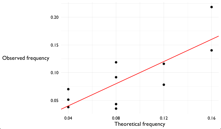
I hope you can see that the observed frequencies are somewhat like the ones predicted by the model. But there's still a fair bit of variation. There could be two causes:

• Maybe we're seeing sampling variation (if we generated more samples, maybe it would start to look more similar). Or
• Maybe the real dice really are different to the model, we just haven't detected it yet!

To look for the latter we'll go and compute a P-value next.