Computing the (log)likelihood

Inference should be easy, shouldn't it? We just need Bayes' theorem:

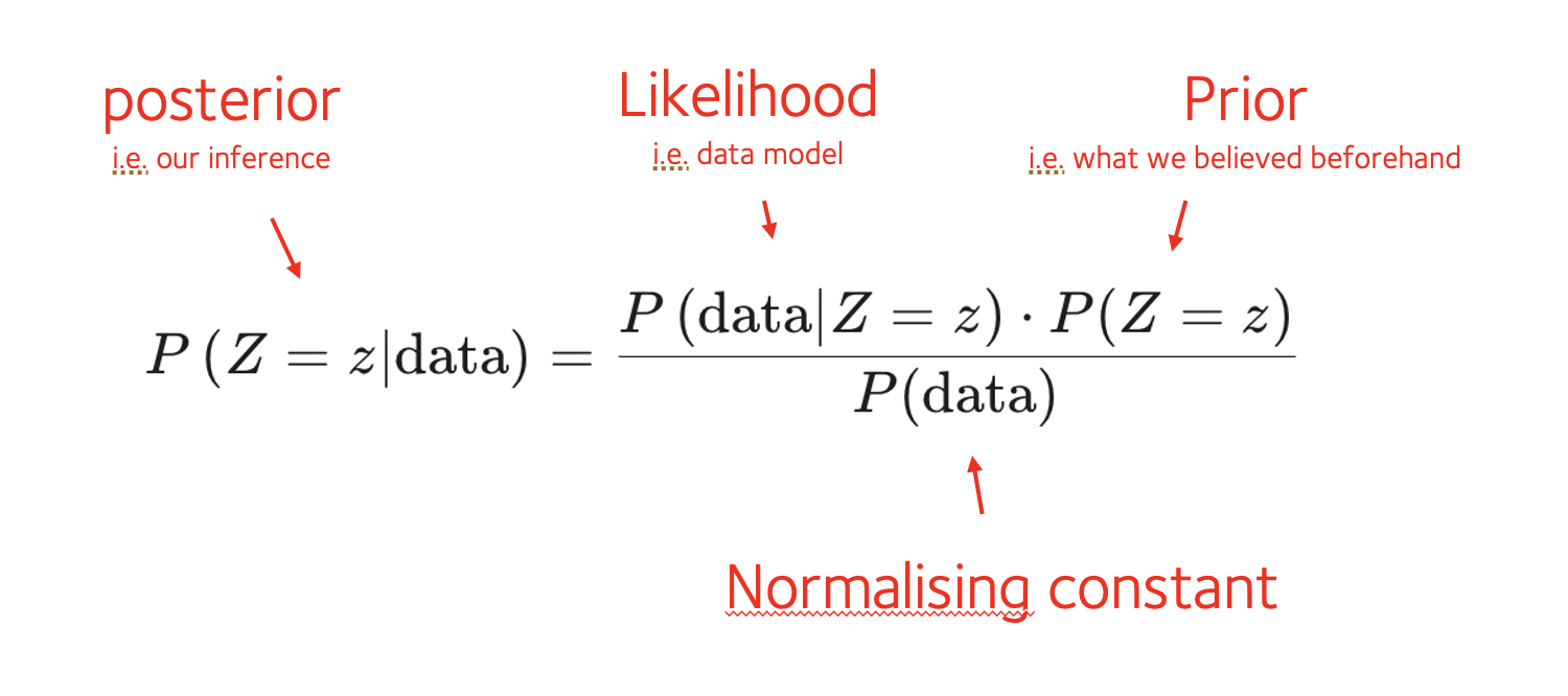
To use it we'll work like this:

1. We'll set $Z$ to mean 'our model fo the dice', with different models representing the blu-tack possibilities.

2. We'll then compute a likelihood of each model.

3. We'll multiply by a prior probability..

4. and we'll renormalise to compute the posterior probability for each model.

Whichever is most likely, must be our model.

Sounds easy! Let's try now.

The likelihood

First let's create a likelihood function - the probability of the data given the model, for any given model of the dice.

Luckily, you've pretty much got this already! Remember that function two_dice_likelihood() that we happened to call 'likelihood' earlier? Turns out this does the job for us.

For example, for a fair die model:

fair_die_model = rep( 1/6, 6 )
two_dice_likelihood( data$sum_of_dice, fair_die_model )

Yay! Lots of probabilities!

Independence day

Hmm. Ok, that produces one probability value per roll. What we really want is the overall probability of the data.

How should we combine probabilities? Well, we have an important thing to work with: the seperate dice rolls are independent of each other and therefore we ought to be able to multiply probabilities

$$P(\text{roll 1}, \text{roll 2}, \text{roll 3}, ... ) = P(\text{roll 1}) \times P(\text{roll 2}) \times \cdots$$

Note

Well, this isn't quite right. For two reasons.

1. Firstly, the dice have blu-tack on. So they're going to avoid similar numbers each time.
2. Secondly, the dice have blu-tack on! Which could for example be getting dented on each roll, affecting the next roll.

Let's imagine the second effect is relatively minor (I can confirm the blu-tack stayed on, at least), what we can probably safely assume is that they are approximately independent given the side the blu-tack is on.

If $B$ denotes 'which side the blu-tack is on', we could write this as:

$$P( \text{roll 1}, \text{roll 2}, \cdots | B ) \approx P( \text{roll 1} | B ) \times P( \text{roll 2} | B ) \times \cdots$$

Luckily $B$ is exactly the model we are calculating the likelihood for! So the upshot is yes we can just multiply the probabilities across the different dice rolls.

(If you are not used to this way of thinking you need the probability cheatsheet.)

Notation note

In probability symbols, we use a vertical bar $|$ to mean 'given', so for example:

• $P(\text{it's cloudy} | \text{it's raining})$
• $P(\text{statistics is fun} | \text{it's bayesian})$

and so on.

To make things sound more exciting, statisticians also sometimes say "conditional on" instead of "given".

The overall likelihood

So let's try:

# Function to compute overall likelihood
total_likelihood = function( sum_of_dice, die_model = rep( 1/6, 6 ) ) {
    prod(
        two_dice_likelihood( sum_of_dice, die_model )$probability
    )
}

Before running this function on the data - stop for a minute and think what you think the likelihood will be. It's the likelihood of this particular set of dice results, over a run of 30 dice rolls. Will the probability be close to 1? Close to 0? Somewhere in between?

total_likelihood( data$sum_of_dice, fair_die_model )

Uh-oh. If you look at the value of this you'll see it's tiny. (How tiny?)

This is in fact typical of real data models, and is expected. After all, for our set of 30 dice rolls, there are

$11^{30} = 1.7\times 10^{31}$

possible outcomes. And we are looking at the probability of just one of them. No wonder the number is small.

Log space warning

Warning

What's happening is we are multiplying lots of small numbers here (lots of probabilities < 1).

It's working but we're at risk of the computer running out of precision and underflowing. Indeed if the number of data points was larger - say 100, or 1,000, our function would probably fail. (The probabilities would get so small the computer couldn't keep track.)

For this reason it is generally better to compute a log-likelihood.

The overall log-likelihood

To better deal with tiny numbers we are going to switch to working in 'log space' - that is, working with log probabilities.

It works like this. Here is a graph of $\log(x)$ over the range of probabilities $[0,1]$:

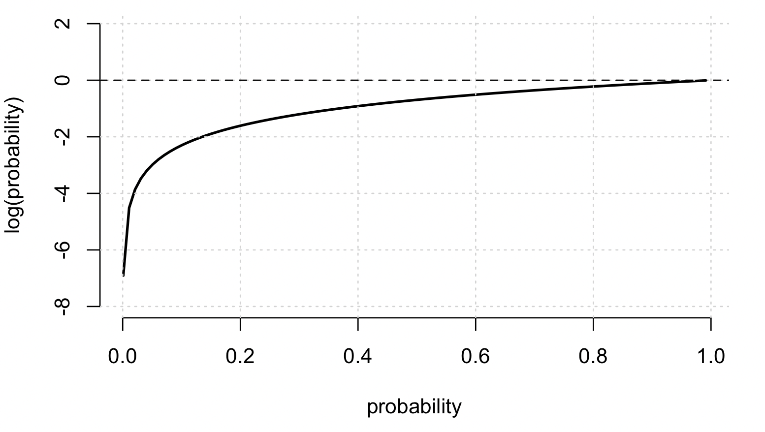
The log transformation has three key properties:

1. probabilities get converted to negative numbers between $-\infty$ and $0$.
2. Tiny numbers (like $10^{-30}$) get converted into large, but not that large negative numbers (like $-70$). They become more numerically manageable numerically.
3. And multiplication of probabilities corresponds to addition of log-probabilities.

For these reason it is common to represent probabilities in log space and then use addition of log probabilities instead of multiplication of probabilities. So let's do that instead:

total_loglikelihood = function( sum_of_dice, die_model = rep( 1/6, 6 ) ) {
    sum(
        log(
            two_dice_likelihood( sum_of_dice, die_model )$probability
        )
    )
}

Question

For example, what's the loglikelihood under a model where $4$ is omitted? (E.g. c( 0.2, 0.2, 0.2, 0, 0.2, 0.2 ))

What about 5?

Why is this happening?