Simulating two dice rolls

Basic dice simulation

Let's write code to simulate rolling two dice - and plot it.

The sample() function is a very helpful R function that (as its name suggests) lets you sample from a set of things.

For example to 'roll' one dice in R, we could just sample possible results. E.g. let's roll a dice 100 times:

sample( 1:6, size = 100, replace = TRUE )

To sample two dice... we could just do it twice:

sample( 1:6, size = 100, replace = TRUE ) + sample( 1:6, size = 100, replace = TRUE )

Note

You need replace = TRUE here because you can't sample 100 things from only 6, unless you replace each one you pick!

Let's make that a reuseable function:

simulate_two_dice <- function( number_of_rolls ) {
    die1 = sample( 1:6, size = number_of_rolls, replace = T )
    die2 = sample( 1:6, size = number_of_rolls, replace = T )
    return(
        tibble::tibble(
            roll = 1:number_of_rolls,
            sum_of_dice = die1 + die2
        )
    )
}

Try running it a couple of times - looks good?

Visualising it

To convince ourselves this is working, let's try plotting a histogram.

Note

A histogram is a simple, data-based estimate of a distribution. It separates values into a set of bins and then plots the counts, or frequencies in each bin.

A basic function to do this in R is hist().

simulation = simulate_two_dice( 100 )
hist( simulation$sum_of_dice )

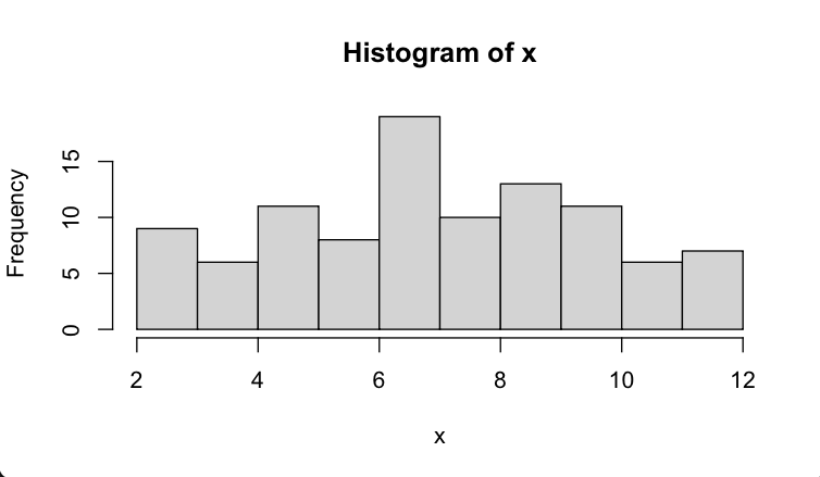
It can look slightly better if we specify 'breaks' to tell the histogram function how to bin values:

breaks = (2:13)-0.5 # 'breaks' between histogram values
hist( simulation$sum_of_dice, breaks = breaks )

We could also compute the sample mean and sample variance:

mean( simulation$sum_of_dice )
var( simulation$sum_of_dice )

Hmm. Is the simulated distribution similar to the theoretical distribution we worked out in class? Not particularly.

Try more rolls!

What happens if we increase the number of rolls?

simulation = simulate_two_dice( 10000 )
hist( simulation$sum_of_dice, breaks = my_breaks )

Hmm.

Note

How far off are the mean, or variance in the simulation? Use mean() and var() to find out - you can compare to your earlier computation.

Of course that's just one simulation. Here's a bit of code that will instead run 10,000 simulations, each with 100 rolls of two dice, 10,000 times over, to find out how much they vary:

variation = (
    tibble::tibble( attempt = 1:10000 )
    %>% group_by( attempt )
    # reframe() is like summarise(), but you can return multiple values:
    %>% reframe(
        simulate_two_dice( number_of_rolls = 100 )
    )
    %>% group_by( attempt )
    %>% summarise(
        mean     = mean( sum_of_dice ),
        variance = var( sum_of_dice )
    )
)

hist( variation$mean, xlim = c( 2, 12 ) )

hist( variation$variance, xlim = c( 2, 12 ) )

Hmm. You'll probably find this sample mean varies from about $6$ to $8$, and the sample variance from about $3$ to $9$. The true distribution mean and variance were 7 and 5.83, so they are in the right ballpark.

(What about if you increase the number of rolls?)

Digression: plotting using ggplot

As an aside - maybe you prefer ggplot?

library( ggplot2 )
(

)
simulation = 
print( simulation )

p = (
    ggplot( data = simulate_two_dice( 10000 ))
    + geom_histogram(
        aes( x = sum_of_dice ),
        breaks = (2:13)-0.5
    )
    + theme_minimal()
)

print(p)

A better ggplot

Hmm. In a complete digression, to make it better I'll also set a nicer theme:

mytheme = function( fontsize = 16 ) {
    (
        theme_minimal( base_size = fontsize, base_family = "gill sans" )
        + theme(
            axis.title.y = element_text( angle = 0, hjust = 1, vjust = 0.5 )
        )
    )
}

And also add an X scale and some axis labels:

p = (
    ggplot( data = simulate_two_dice( 10000 ))
    + geom_histogram( aes( x = sum_of_dice ), breaks = (2:13)-0.5, colour = 'black' )
    + scale_x_continuous( breaks = 2:12 )
    + xlab( "Sum of dice" )
    + ylab( "Count" )
    + mytheme()
)
print(p)