How to interpret the P-value

So you've done a statistical test, got an estimate, a standard error and a P-value. How do you know when there's enough evidence for you to start thinking the effect might really be there? This part of the tutorial will walk you through the main ways to think about this problem.

Example

For example, in our linear regression example we observed a possible association between the genotypes of a SNP in the gene ATP2B4 and expression of ATP2B4. The fitted coefficients (including a covariate, stage) were:

               Estimate  Std. Error   Pr(>|t|)
(Intercept)      0.0447      0.0165     0.0131
dosage           0.0392      0.0109     0.0017
stagefetal      -0.0477      0.0124     0.0009

So the estimate $\hat{\beta}$ of the effect of the genotype dosage $\beta$ is 0.0392, and the P-value is 0.0017. Is this enough evidence to conclude that the effect is nonzero?

A sanity check

Before getting started - note that by even asking this question we are making a key assumption - that it's sensible to try to discern 'true' effects from 'zero' effects.

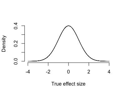
Suppose genetic effects on expression actually follow a continuous distribution - say, a gaussian-like distribution where there are many small effects and a few larger ones:

Here essentially all effects are nonzero. It is pointless to ask whether one of them might be nonzero.

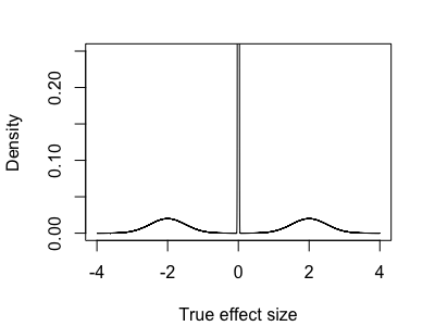
On the other hand, maybe most variants have no effect at all, or very small effects, and a few have large effects - something like:

Here it definitely makes sense to try to call some effects as 'nonzero' - with enough data we ought to be able to distinguish those effects out in the tails.

In many problems - such as looking for genetic variants that affect gene expression - it seems likely though that the real distribution might be a kind of mixture between these two. For example there might be:

• lots of variants across the genome that don't affect expression at all

• a small number of variants in gene promoter regions that strongly affect expression.

• a number of more variants in more distant enhancer regions, that might perhaps have substantial but more modest effects.

• and of course expression is affected by many other factors, such as chromatin accessibility and the availability of relevant transcription factors. So in principle there might be a large set of variants in other parts of the genome that also affect expression to a more limited extent.

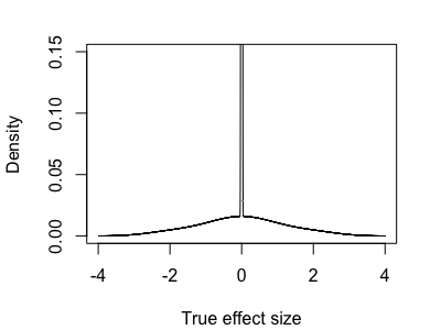
So the true distribution of real effects might look something like:

In this case we are in a kind of half-way house - it sort of makes sense to try to distinguish the zero effects from the nonzero ones, but we have to be aware we'll also be calling many small-but-nonzero effects as zero as we do it.

With this warning aside, for the rest of this page I'll assume we are happy to try to ask whether $\beta$ is nonzero - that is, we are assuming a 'mixture' model where some effects are zero and some aren't. To make this concrete, we'll assume:

• that truly nonzero effects $(\beta \neq 0)$ come along at some frequency $\Pi$, and

• The strength of the truly nonzero effects are distributed according to some distribution $\beta \sim \Omega$.

(For example, the mixtures depicted above had 95% of the mass on the 'spike' near zero and $5% on a diffuse distribution centred at zero.)

With this model, it makes sense to try to find those truly nonzero effects.

How small a p-value is needed to be convinced?

So we've done our study and got a P-value. How small does this need to be before we can be reasonably convinced our effect is nonzero?

A standard way to approach this is to seek a threshold $\alpha$ such that if the p-value is smaller than the threshold

$$p < \alpha$$

then the effect is likely to be genuinely nonzero - that is, we would like

$$P(\beta\neq 0 | p<\alpha )$$

to be large.

The expression above can be computed this using Bayes' rule:

$$P(\beta\neq 0 | p < \alpha) = \frac{P( p < \alpha | \beta\neq 0 )\cdot P(\beta \neq 0)}{P(p < \alpha)}$$

The terms on in the above formula have specific names:

• $P(p<\alpha|\beta\neq 0)$ is the statistical power - it's the chance of detecting a truly nonzero effect.

• $P(\beta\neq 0)$ is the probability* that the effect is truly nonzero before we've seen any data. Recall that in our mixture model of effects this was denoted $\Pi$.

If we include these and expand the denominator we get the key formula for p-values:

Key formula (probability version)

$$P(\beta\neq 0 | p < \alpha) = \frac{\text{power} \cdot \Pi}{\text{power}\cdot\Pi + \alpha\cdot(1-\Pi)}$$

Note. That still looks a bit complex. A slightly simpler version can be given by working on the odds scale instad of the probability scale. (Remember that if $x$ is a probability, the odds correponding to $x$ is $\frac{x}{1-x}$). On the odds scale the formula becomes:

Key formula (odds version)

$$\text{odds}(\beta\neq 0 | p < \alpha) = \frac{\text{power}}{\alpha} \cdot (\text{prior odds})$$

where

$$\text{prior odds} = \frac{\Pi}{1-\Pi}$$

This formula makes clear that choice of a reasonable threshold for the P-value depends on the interplay between the study power and the prior probability (or odds) of the effect.

Given that we are happy to assume the mixture model of effects outlined above (that is, such that the question 'is $\beta \neq 0$' makes sense), the formula tells us how to pick p-value thresholds to have good condfidence that our 'discoveries' represent real associations.

Note

The left hand side of the key formula can be called the "posterior probability (or odds) of association" given $p<\alpha$.

Another name for it is the positive true discovery rate given $p < \alpha$. This naming comes about by analogy to the 'positive false discovery rate' which is effectively defined as one minus the quantity above:

$$\text{pFDR}(p<\alpha) = P(\beta = 0 | p < \alpha)$$

Interpreting evidence

The key formula gives us a way to pick a sensible p-value threshold $\alpha$. To apply it you have to know two things:

• the power of the test

• the prior probability $\Pi$

There are three ways to work these out. Either

1. you can make them up.
2. you can learn them from other, previously published datasets.
3. or you can try to learn them from the dataset itself.

All three of these approaches can be useful.

Example: the WTCCC GWAS paper

The 'key formula' appears in Box 1 of the original Wellcome Trust Case-Control Consortium paper, which was one of the earliest large genome-wide association studies. It was used to pick a threshold of $\alpha = 5\times 10^{-7}$ for following up on putative genetic associations.

Here's how the calculation was presented. The authors supposed there might be, heuristically, around a million 'linkage disequilibrium blocks' in the human genome. (A linkage disequilibrium block is a region of the genome, perhaps bordered by recombination hotspots, over which common genetic variants have become correlated due to ancestral processes such as genetic drift). And they supposed that, perhaps, 10 such regions in the genome might be genuinely associated with a given common disease - giving an approximate prior odds of

$$\frac{\Pi}{1-\Pi} \approx 10^{-5}$$

If the power were around 50% then this would give

$$\text{odds}(\beta\neq 0 | p < \alpha) = \frac{0.5}{\alpha} \times 10^{-5}$$

If $\alpha = 5\times 10^{-7}$ then

$$\text{odds}(\beta\neq 0 | p < \alpha) = \frac{5\times 10^{-1}}{5\times 10^{-7}} \times 10^{-5} = 10$$

So - if the assumptions are right - $p < 5\times 10^{-7}$ should give us a posterior odds of 10, or a posterior probability of about a 90% that the association is truly nonzero.

Now obviously these values are made up - the prior probability estimate could have been wildly out of range, and the true power wasn't known either. Nevertheless, this heuristic calculation, which was based on the core hypothesis about the genetic architecture of common diseases, provided a useful and defensible threshold. In practice it worked well and led to key new findings which were later replicated in other studies.

Example - estimating the discovery rates

John Storey's 2001 paper introduced the idea that - if we have conducted lots of similar tests - the quantities $\Pi$ and the power can be estimated from the data itself. The proposed approach goes something like this. Suppose we have conducted $M$ tests (of independent hypotheses) with P-values $p_1,\cdots,p_M$. To apply our formula, we'd need to know both the power and the true proportion $\Pi$ of true positives. However, if $M$ is large we might be able to estimate them as follows:

• Tests with p-values greater than (say) $\lambda = \frac{1}{2}$ probably reflect the null model - i.e. those where the true effect is zero. And P-values for null tests should be uniformly distributed. So, we could estimate $\Pi$ as the excess in small p-values over what we'd predict from the number of large p-values:

$$\Pi \approx 1 - \frac{ \# \{p_i|p_i > \lambda\} } {(1-\lambda)M}$$

• We can't estimate the power directly, but could take

$$P(p_i<\alpha) \approx \frac{\# \{p_i|p_i < \alpha\}}{M}$$

Combining with the above estimate $\hat{\Pi}$ of $\Pi$ gives

Plugging these in leads to the positive false discovery rate estimate:

$$P(\beta=0|p<\alpha) = \frac{\alpha}{1-\lambda} \cdot \frac{ \#\{p_i|p_i>\lambda\} } { \# \{p_i|p_i < \alpha\} }$$

and of course the corresponding true discovery rate $P(\beta\neq 0|p<\alpha)$ is one minus this quantity.

Storey's FDR method therefore provides a way to estimate the key quantities in the key formula from the data itself - provided we have lots of data to work with.