Quantiles, p-values and all that

Consider a variable $X$ that is normally distributed - here is a picture of its distribution:

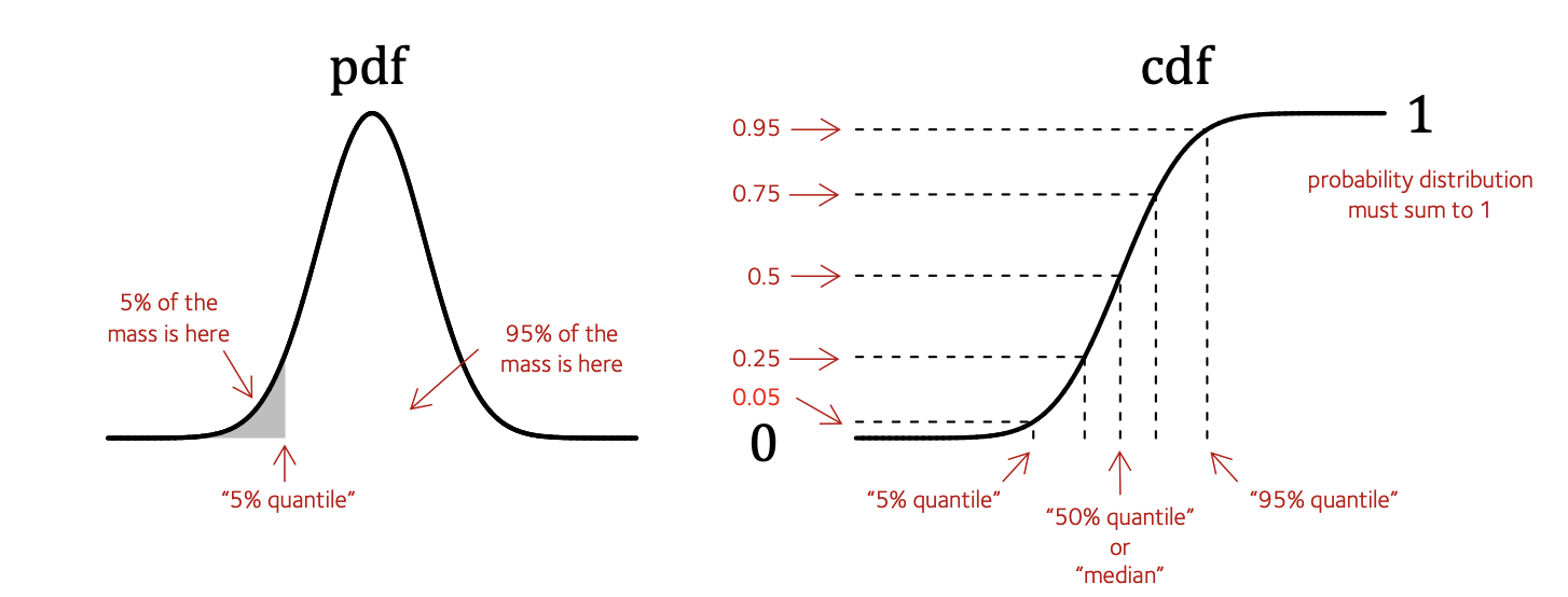
I've annotated this with various pieces of information.

On the left is shown the probability density function or pdf. You could compute this using dnorm() in R as we did on this page.

To fix terminology I've labelled a particular point on the X axis - the $5\%$ quantile. That means: the value $x$ such that exactly 5% of the mass of the distribution is $\leq x$.

On the right is shown the cumulative density function or cdf. You can compute using pnorm() in R. The cdf is just worked out by summing up (that is, integrating) the area under the pdf from left to right.

Note

Since this is a distribution, the total area under the distribution is $1$. That means the cdf must asymptote to $1$ on the right - look, it does!

Quantile levels and p-values

As the red annotations indicate, the cdf is the function that maps values of $X$ and tells you which quantile they correspond to - i.e. how much mass is to the left of them. For example:

Question

Use pnorm() to answer: for a normal distribution with mean 10 and standard deviation 3, how much of the probability mass is $\leq X=1$?

Hint. If stuck, check the help page to see how to use it. In particular pnorm uses the name q (for 'quantile') instead of x.

What's a p-value?

A p-value is essentially just the same thing as the cdf - but usually applied to a particular observation.

Definition

If a variable $X$ is assumed to have a given distribution, and we observe a value $x$, the P-value corresponding to $x$ is just the mass under values 'at least as extreme' as $x$.

I hope you can see the the way to compute a P-value is $\text{cdf}(x)$.

However we do get a bit of leeway in this definition to fit this to our purpose, depending on what we want to capture by 'more extreme'. For example:

• If values less than $x$ are considered 'more extreme', we might compute:
  $$\text{P-value} = \text{cdf}(x)$$

• If values greater then $x$ are considered 'more extreme', we might instead compute the upper tail probability which is one minus the lower tail:
  $$\text{P-value} = 1 - \text{cdf}(x)$$

Note

In R, you can compute this directly by adding lower.tail = FALSE in your pnorm() call.

• We might be thinking that values greater than $x$ in magnitude are 'more extreme', in which case we'd take something along the lines of:

$$\text{P-value} = \text{cdf}(x) + \left(1-\text{cdf}(-x)\right)$$

This is a 'two-tailed' p-value which picks up both tails of the distribution.

Finding quantiles

You might also want to go the other way: that is, finds the value of $X$ corresponding to a given quantile (such as 5% or 25%). This is the job of the quantile function. If you look at the right-hand diagram above, you'll see that the quantile function is just the inverse of the cdf (it maps the y axis values back to the x axis).

Question

Use qnorm() to answer: For a standard normal distribution (with mean 0 and standard deviation 1), what's the 2.5% quantile at?

Hint. Again, the help page might help. qnorm() uses the name p for the choice of quantile, eg. p=0.025 in the above.

How does the 2.5% quantile change as you change the standard deviation?