Distributions

In statistics, the way uncertainty is accounted for is through probability distributions.

Suppose we are interested in a variable $X$. A distribution for $X$ is just a function that distributes a total of 100% probability 'mass' over the possible values of $X$.

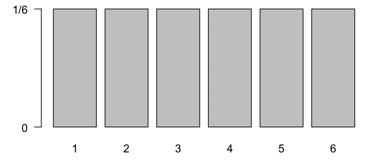
For example, here is the distribution of the roll of a normal 6-sided die:

The die has $6$ possible outcomes $X=1,\cdots,6$, and the function assigns probability mass $\tfrac{1}{6}$ to each of them. Across all possibilities it adds up to $1$ (i.e. $100\%$ total probability.) Simple, right?

Simple distributions like this one can often be worked out just by counting possibilities. For example, let's warm up with an exercise:

Question

What is the distribution of the sum of two dice rolls? Use a pen and paper to draw it.

Hints

This can be worked out just by counting the possibilities. For example, there are $4$ possible dice rolls that generate the value $5$, and there are $36$ possible dice rolls in total. So there ought to be $\tfrac{4}{36} = \tfrac{1}{9}$ chance of rolling a $5$.

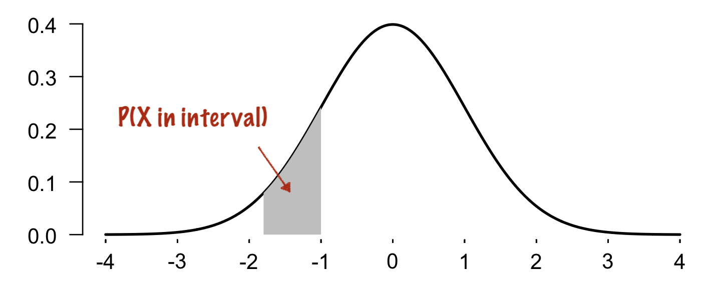
For a continuous variable $X$ things are slightly more complicated because to get an actual probability we typically have to think in terms of ranges of values. For example, here is the density of a normal distributed variable:

Like the dice example, the function sums to $1$ over the whole real line. As shown on the plot, to read off the probability that $X$ is in any given part of its range, we just sum up (integrate) the density over the range. (So the density function itself isn't returning a probability at each point - the probability of any specific value is vanishingly small) - but something that sums up to a probability over any range of values).