The most important formula in science

The most important formula is... Bayes theorem!

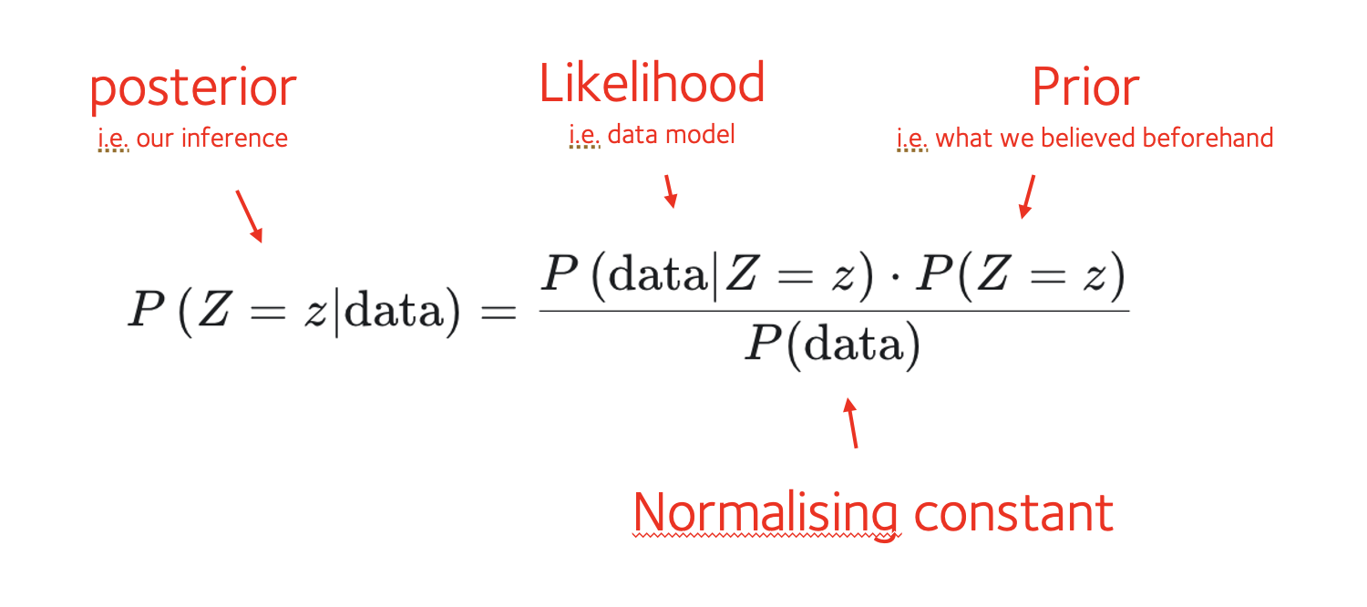
Let's write it now. Suppose $Z$ is something we care about - say, a scientific theory, or the chance of having disease. We collect some data to tell us about it. Bayes' theorem now tells us that:

$$P\left(Z=z|\text{data}\right) = \frac{P\left(\text{data}|Z=z\right) \cdot P(Z=z)}{P(\text{data})}$$

Bayes formula tells us how to update what we should believe about $Z$, given some new data:

• The left-hand side $P(Z=z|\text{data})$ represents our new belief (distribution of $Z$ given the data).
• The right-hand side involves a model for the data $P(\text{data}|Z=z)$, and a term $P(Z=z)$ representing what we used to believe about $Z$ before we saw the data. (There's also a denominator, which like for other distributions acts as a normalising constant. We'll come back to this below.)

The pieces of Bayes' theorm have specific names and interpretations in statistical analysis, as follows:

Using Bayes in practice

In principle, it's easy to use Bayes. We do this:

1. Collect some data about $Z$.
2. Write down a model of the data (the likelihood function).
3. Work out what prior information we have about $Z$.
4. And then apply the formula.

In pratice this can be easy or difficult, depending on how complicated it is to define the likelihood and prior. We'll do some examples in a moment to make this clear.

The denominator

You might be thinking - what's that denominator, why is it a 'normalising constant' - and how would you compute it?

Here are a few things to note:

1. The denominator is 'constant' in that it does not depend on $Z$. (There's no '$Z$' in $P(\text{data})$).

2. Like all distributions, the posterior distribution is supposed to sum to $1$ over possible values of $Z$.

3. The denominator is just the value needed there to make the posterior sum to $1$ over all possible values of $Z$.

The denominator therefore plays the same role as 'normalising constants' for other distributions.

Computing the denominator

So how do we compute the normalising constant? Here are a few things to note.

First, in some settings, where we're only interested in relative values of the posterior for different values of $Z$, we might not need to compute the denominator at all. Its only job is to normalise things into absolute probabilities.

Second, in many problems everything works out 'analytically', meaning that the mathematical form of the posterior is already known - nothing more needed to compute. (For example, the posterior might be a beta distribution or a normal distribution).

Lastly, we can always compute the denominator by summing the numerator over all the possible values of $Z$. In other words, we write it out using the law of total probability:

$$\text{denominator} = P(\text{data}) = \sum_y P\left(\text{data}|Z=y\right) \cdot P(Z=y)$$

For a continuous variable $Z$, this would be an integral.

We'll do some examples of both these methods in a moment.

caution

Working out this sum can sometimes be harder. In this case computational methods like Markov Chain Monte Carlo (MCMC), Laplace approximations or Variational approximations are typically needed. Although these sound complicated, they're really just numerical ways to compute this denominator, and there are plenty of easy-to-use tools to do this.

We won't get into these for now because there are plenty of useful examples where they aren't needed.