Julia
Julia is an interesting language that is pretty good for many data analysis and computational tasks. Like python it has a rich ecosystem of data analysis packages but it has a few features that make it different from others
- like C++ it is strongly typed and compiled. It's easier to avoid paying a performance cost than in python or R.
- Nevertheless it acts much like an interpreted language, like Python or R.
- It also has an interesting approach based on multiple dispatch (different, say, from object-oriented languages like python)
Installing Julia
Installing julia is easy using conda:
mamba install -c conda-forge julia
Or by downloading directly from the julia website. (Note. As before, on Windows you will likely want to install into your UNIX terminal instead - using conda is simplest for that.)
Once installed you can start it by typing julia:
$ julia

               _
   _       _ _(_)_     |  Documentation: https://docs.julialang.org
  (_)     | (_) (_)    |
   _ _   _| |_  __ _   |  Type "?" for help, "]?" for Pkg help.
  | | | | | | |/ _` |  |
  | | |_| | | | (_| |  |  Version 1.7.2 (2022-02-06)
 _/ |\__'_|_|_|\__'_|  |  Official https://julialang.org/ release
|__/                   |

julia>
See the Julia webpage for more details.
Trying it out
To test it, let's try a few things. For example we could create a string variable:
julia> a = "Hello, this is a string"
...or split it into words:
julia> words = split( a, "," )
...or count their lengths:
julia> map( length, words )
To go a bit further, let's install some packages. Press ] to enter the Julia package manager. The prompt should
change to something like this:
(@v1.8) pkg>
Add the Plots and Distributions packages (this might take a few minutes):
(@v1.8) pkg> add Plots, Distributions
    Updating registry at `~/.julia/registries/General.toml`
   Resolving package versions...
   Installed xkbcommon_jll ─ v1.4.1+1
  No Changes to `~/.julia/environments/v1.8/Project.toml`
    Updating `~/.julia/environments/v1.8/Manifest.toml`
  [d8fb68d0] ↑ xkbcommon_jll v1.4.1+0 ⇒ v1.4.1+1
Precompiling project...
  6 dependencies successfully precompiled in 44 seconds. 283 already precompiled.
To get out of package mode again, press <backspace> (or ctrl-C.).
The add command has installed the packages but not imported them into our local session.
To tell julia we want to use them, use using:
julia> using Plots, Distributions
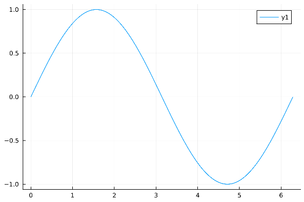
Now we can make some simple plots, rather similar to the ones we made in R:
x = 0:0.01:2 * pi
y = sin.( x )
plot( x, sin.( x ))

Note
The . after sin is not a mistake - it's actually a julia feature which expands the use of a function (sin())
across an array of numbers.
In R we didn't need this - it happens automatically with many functions. But it can also get awkward when you reach a
function that doesn't work on vectors like this (as sometimes happens when you are writing code).
The julia approach is actually often nice - you write the function once, operating on one number, and then to apply it across
arrays you use the ..
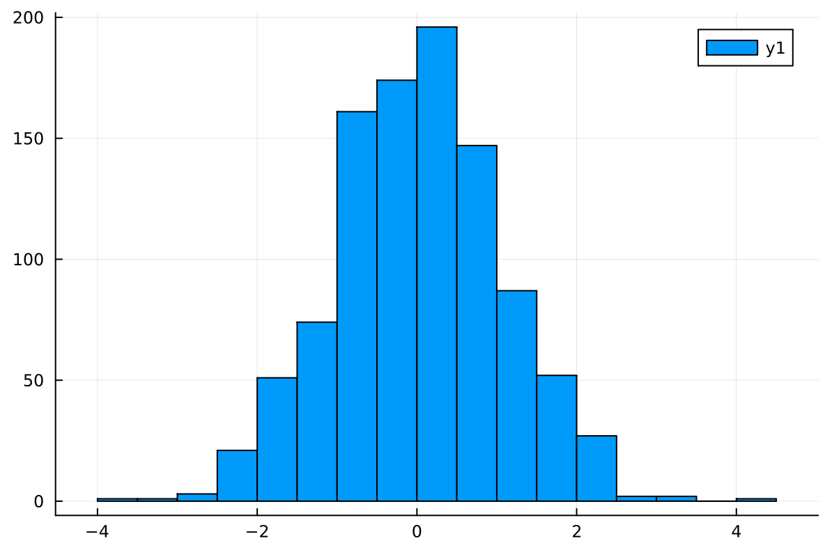
Or we can generate and plot a million samples from a Gaussian distribution:
data = rand( Normal(0, 1), 1000 )
histogram( data, bins = 25 )

Getting help
Julia also has a great help system - type ? to get into the built-in help, then search for a topic such as histogram.
Next steps
Like R and python, perhaps the nicest way to use julia for interactive work is through JupyterLab. See how to install Jupyterlab for details.