A naive approach

Figuring out the proportion in genes should be pretty easy using the dplyr data verbs, right?. We could

1. group genes by species and chromosome
2. compute the total length by summing
3. join to the contigs dataset to compute total chromosome/region length
4. and then summarise.

Here's a function that does 1-3 above:

compute_lengths_per_chromosome = function(
   data,
   chromosomes = contigs
) {
   (
      data
      # Group by species / chromosome
      %>% group_by( dataset, seqid )
      # Add up the gene lengths
      %>% summarise(
         number_of_genes = n(),
         total_gene_length = sum( end - start + 1 )
      )
      # Add the chromosome lengths
      %>% left_join(
         chromosomes[, c( "dataset", "seqid", "attributes", "sequence_length" )],
         by = c( "dataset", "seqid" )
      )
   )
}

The idea is that this has both a 'total gene length' (sum of lengths of genes) and the total sequence length (length of the chromosome or contig) in the same dataframe:

You can use it like this:

print( compute_lengths_per_chromosome( genes ) )

# A tibble: 5,469 × 6
# Groups:   dataset [11]
   dataset    seqid number_of_genes total_gene_length attributes sequence_length
   <chr>      <chr>           <int>             <dbl> <chr>                <dbl>
 1 Acanthoch… MVNR…              56           1349511 Alias=orp…         2466117
 2 Acanthoch… MVNR…              39           1029333 Alias=orp…         2338421
 3 Acanthoch… MVNR…              56           1399228 Alias=orp…         2213793
 4 Acanthoch… MVNR…              41           1113000 Alias=orp…         2013838
 5 Acanthoch… MVNR…              45           1012078 Alias=orp…         1950346
 6 Acanthoch… MVNR…              54            989013 Alias=orp…         2094391
 7 Acanthoch… MVNR…              84           1074990 Alias=orp…         1729193
 8 Acanthoch… MVNR…              72           1486459 Alias=orp…         2368326
 9 Acanthoch… MVNR…              50           1237060 Alias=orp…         2396890
10 Acanthoch… MVNR…              39            643138 Alias=orp…         1656807

And all we have to do is step 4 - sum them up across chromosomes:

naive_proportions = (
   compute_lengths_per_chromosome( genes )
   %>% group_by( dataset )
   %>% summarise(
      total_gene_length = sum( total_gene_length ),
      total_genome_length = sum( sequence_length )
   )
   %>% mutate(
      proportion_in_genes = total_gene_length / total_genome_length
   )
)
print( naive_proportions )

# A tibble: 11 × 4
   dataset                                           total_gene_length total_genome_length proportion_in_genes
   <chr>                                                         <dbl>               <dbl>               <dbl>
 1 Acanthochromis_polyacanthus.ASM210954v1.110               422171067           830201259               0.509
 2 Asparagus_officinalis.Aspof.V1.57                         165883925          1015569172               0.163
 3 Bufo_bufo-GCA_905171765.1-2022_05-genes                  1290309576          5003028965               0.258
 4 Camelus_dromedarius.CamDro2.110.chr                       825762826          2052758708               0.402
 5 Gallus_gallus.bGalGal1.mat.broiler.GRCg7b.110.chr         583352821          1041139641               0.560
 6 Homo_sapiens.GRCh38.110.chr                              1379802830          3088286401               0.447
 7 Mus_musculus.GRCm39.110.chr                              1070748851          2723431143               0.393
 8 Pan_troglodytes.Pan_tro_3.0.110.chr                      1110722691          2967125077               0.374
 9 Plasmodium_falciparum.ASM276v2.57                          13776689            23292622               0.591
10 Plasmodium_knowlesi.ASM635v1.57                            12970692            23462187               0.553
11 Plasmodium_vivax.ASM241v2.57                               14052272            23768694               0.591
To figure out how much of the genome is covered by genes, or by exons, we face a problem.
In principle we could just add together the gene lengths.

(
   ggplot( data = proportions )
   + geom_col(
      aes(
         x = proportion_in_genes,
         y = dataset
      )
   )
   + ylab( "Species" )
   + xlab( "Proportion of genome in genes" )
   + theme_minimal(16)
)

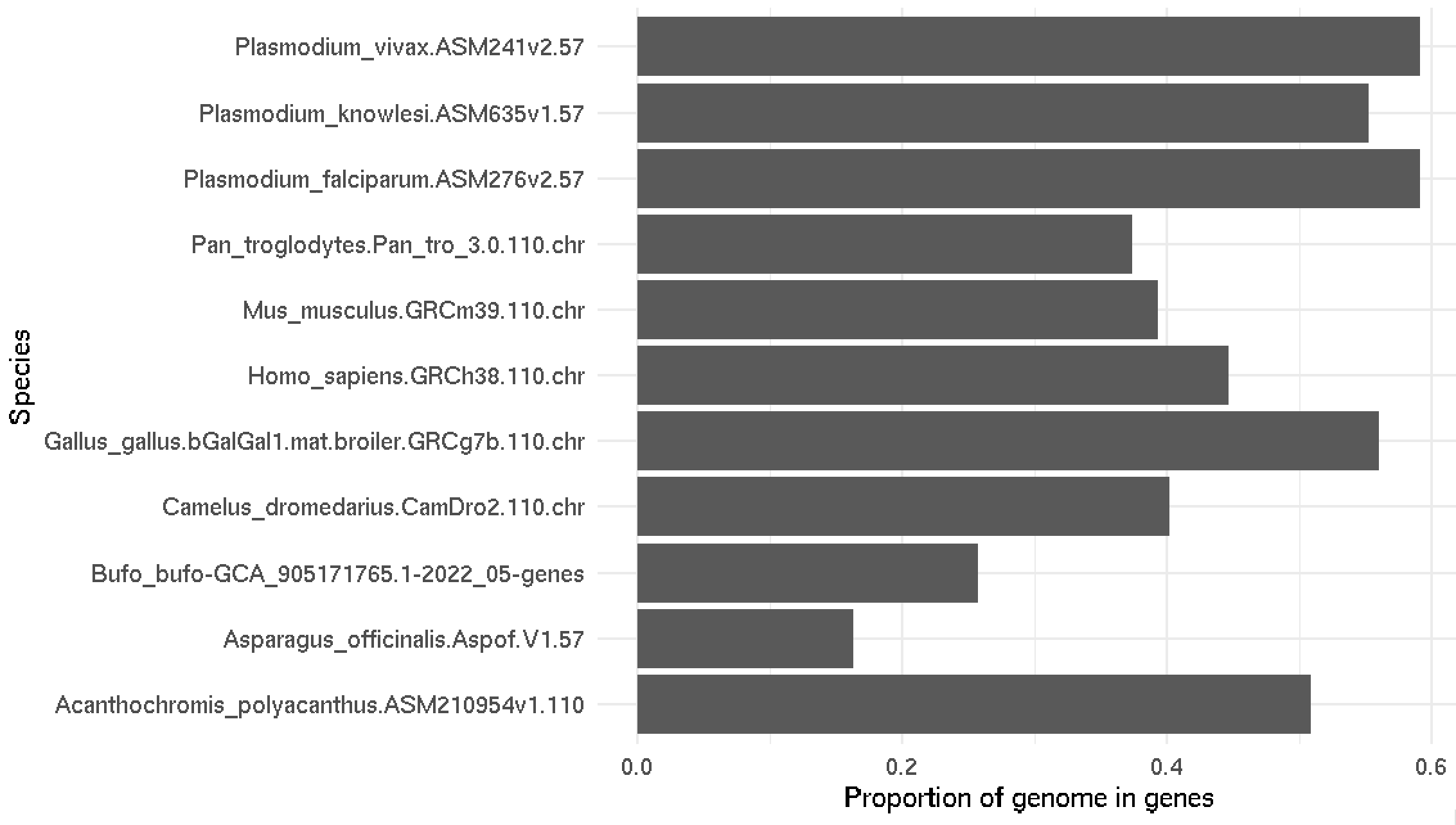
Pretty cool huh! Most species have 40-60% of the genome in genes. Is this right?

However

Unfortunately this calculation is (slightly) wrong. Why?

To get it right, we need to do some more coding...